REU2019: Validation of Higgs to $b\bar{b}$ tagging techniques with $Z\rightarrow b\bar{b}$

Goal

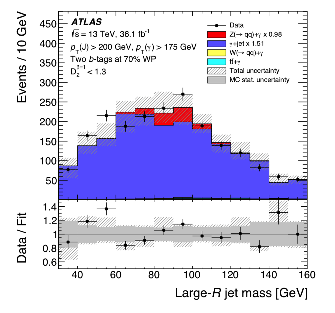
Use $Z\rightarrow b\bar{b}$ process to validate performance of techniques used to identify $H\rightarrow b\bar{b}$.

Data

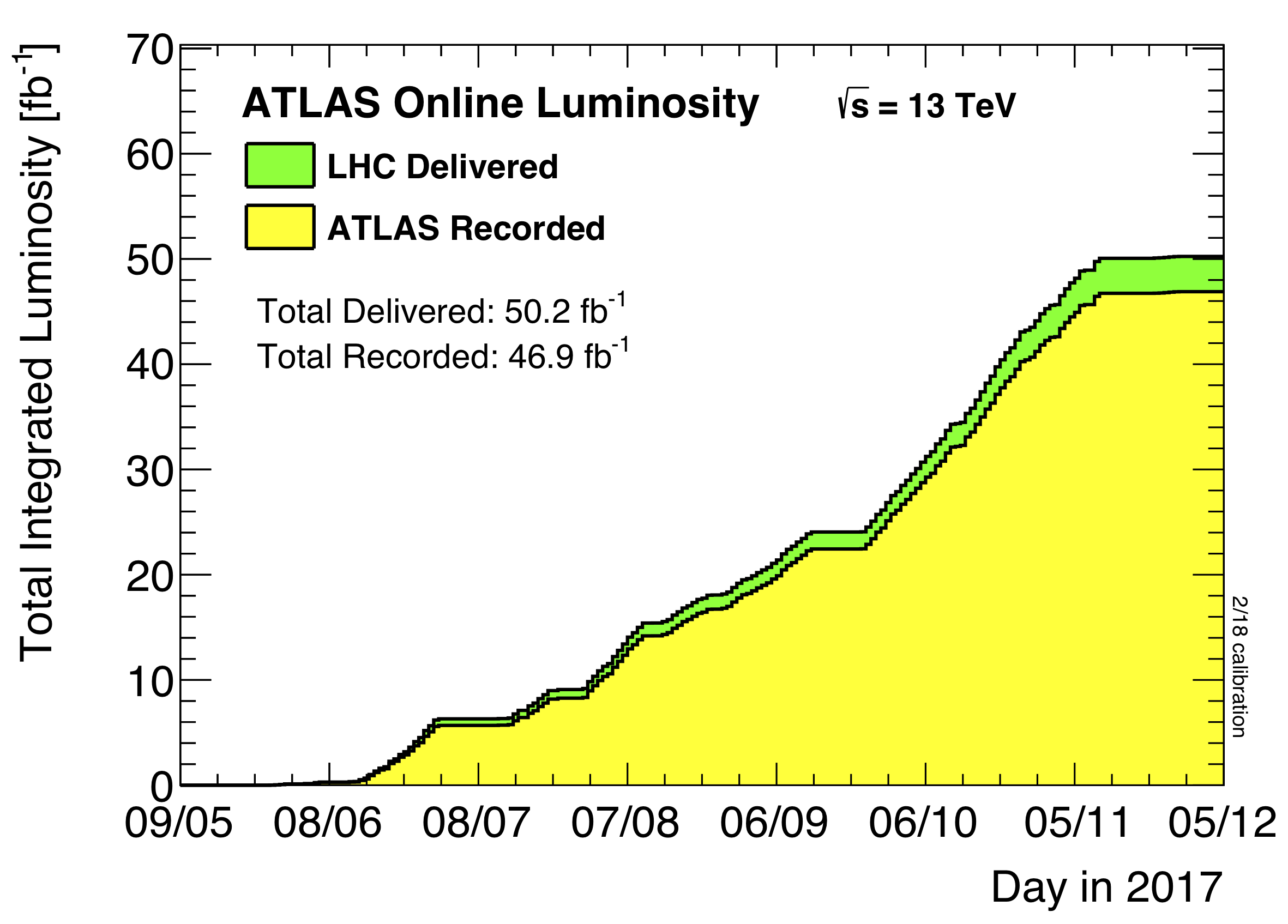
• Proton-proton collisions from the 2017 LHC run, at a centre of mass energy of 13 TeV.
• A total luminosity of approximately $47 \text{fb}^{-1}$ was recorded by ATLAS.

Monte-Carlo samples

• Signal: $Z(\rightarrow b\bar{b})+\gamma$
  

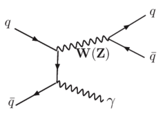
• Dominant background: photon + jets, where the jets contain gluons splitting into pairs of bottom quarks. Examples of leading-order diagrams:
  

• Smaller contributions from $t\bar{t}\gamma$ and $W\gamma$.

• Negligible contributions from jets faking photons, electrons faking photons and $t\bar{t}$.

Event selection

• See this ATLAS paper draft, Section 8:
  • Single-photon trigger: transverse energy above 140 GeV and loose photon identification requirements.
  • Photon with $E_{T}>175$ GeV.
  • Primary vertex and jet-cleaning requiremetns.
  • Exactly one photon and at least one large-R jet with $p_{T}> 200$ GeV, $|\eta|<2.0$, mass greater than 30 GeV.
  • Jet-photon overlap removal: remove photons within $\Delta R=1.0$ of the large-R jet.
  • $Z\rightarrow b\bar{b}$ candidate is highest $p_{T}$ large-R jet.

Ntuples

• Basic pre-selection cuts (defined here and already applied):

  • GRL: select only events on good runs list
  • GOODCALO: ensure that the LAr and Tile are working properly for this event (no noise bursts)
  • PRIVTX: ensure that at least a primary vertex exists in the event.

• Names and physics processes: the ntuples are split by data and simulation (MC). For MC, they are further split by type of process that was generated, with associated dataset IDs:

  • 361039-361062 correspond to photon + jets samples (generated in several bins of transverse momentum).
  • 305435-305439 correspond to W(qq) + photon
  • 305440-305444 correspond to Z(qq) + photon

How to start

1. A code skeleton that reads ntuples and creates histograms of relevant variables is here:

/data/users/miochoa/REU2019/reu-2019-skeleton

2. Copy the entire folder above into your user area in /data/users/<your-username>. If your user area does not yet exist, create it and cd into it, then:
   cp -r /data/users/miochoa/REU2019/reu-2019-skeleton .

3. Everytime you start a session, you need to setup the required tools by running:

cd reu-2019-skeleton
source setup.sh

3. The event and object selection as well as histogram definition takes place here:

ZbbAnalysisCode/src/MyZbbAnalysis.C

Follow the existing examples to add new histograms.

4. How to run a test after any modification:

   cd run/
   root -l -b
   .L runAnalysis.C
   runAnalysis(dataset name, "12", "local")
   

   The “dataset name” should be replaced by one of the datasets listed in:

   run/inputs/data.txt or inputs/mc.txt
   

   This step will produce an output.root file. Inspect it to make sure your histograms are properly filled.

5. How to run on the full list of data and MC samples:

   cd run/
   ./localRun.sh inputs/data.txt
   ./localRun.sh inputs/mc.txt
   

   These two steps will produce output root files for each data or MC sample (around 250). You can combine the root files from data all in a single file, with the following command:

   hadd output_data.root output_data_*root
   

   The MC files can’t be combined, because they will have to be individually scaled by their corresponding cross-sections, which is performed in the next step.

6. There is an example python script for making nice plots with the histograms produced in the earlier steps:

   cd Plotting/
   python new_plotting_example.py -b
   

Questions

1. How are photons identified and reconstructed in ATLAS?
   • E.g. on the paper cited above, a loose photon requirement is mentioned. What does it consist of?
2. This work uses two ‘types’ of jets: large-R calorimeter jets and variable-R track-jets.
   • How are jets defined and built in ATLAS?
3. We also use b-tagging techniques to identify jets that contain b-hadrons: what properties of the b-quark are useful for this tagging?
4. What goes into the scaling of the MC samples before you make your plots?

Studies

1. Study data/MC agreement in different variables and selections:
   • e.g. before and after requiring two b-tagged jets associated to the large-R jet.
2. What is the signal efficiency for different b-tagging selections?
3. Are there distributions that provide discriminant power between $\gamma$+jets and $Z\rightarrow b\bar{b}$?
4. How does the efficiency to find a $Z\rightarrow b\bar{b}$ object in data compare to the efficiency in MC?