(fitting-histogram)=
# Walkthrough: Fitting a histogram (15 minutes)
I created a file with a couple of histograms in it for you to play with.
Switch to your UNIX window and copy this file into your directory:[^f31]
> cp ~seligman/root-class/histogram.root $PWD
Go back to your TBrowser window. (If you've quit ROOT, just start it
again and start a new browser.) Click on the folder in the left-hand
pane with the same name as your home directory.
Double-click on `histogram.root`. You can see that I've created two
histograms with the names `hist1` and `hist2`. Double-click on
`hist1`; you may have to move or switch windows around, or click on
the `Canvas 1` tab, to see the `c1` canvas displayed.
:::{note}
You can guess from the x-axis label that I created this histogram from a
gaussian distribution, but what were the parameters? In physics, to
answer this question we typically perform a "fit" on the histogram: you
assume a functional form that depends on one or more parameters, and
then try to find the value of those parameters that make the function
best fit the histogram.
:::
Right-click on the histogram and select **FitPanel**. Under **Fit
Function**, make sure that **Predef-1D** is selected. Then make sure
**gaus** is selected in the pop-up menu next to it, and **Chi-square**
is selected in the `Fit Settings->Method` pop-up menu. Click on
**Fit** at the bottom of the panel. You'll see two changes: A function
is drawn on top of the histogram, and the fit results are printed on the
ROOT command window.[^fitpanel]
[^fitpanel]: What do all these options mean? The **Fit Function** selects
which mathematical function is going to be used to fit the histogram.
**Predef-1D** means that the function is going to come from one of ROOT's
pre-defined one-dimensional math functions; as you will learn in just a
bit, you can define functions of your own. **Chi-square** refers a fitting
method; for any fit that you're likely to do with a **FitPanel**, this
will be the method you'll use.
(statistics-question)=
:::::{note}
Interpreting fit results takes a bit of practice. Recall that a gaussian
has 3 parameters ($P_0$, $P_1$, and $P_2$); these are labeled
"Constant", "Mean", and "Sigma" on the fit output. ROOT determined
that the best value for the "Mean" was 5.98±0.03, and the best value
for the "Sigma" was 2.43±0.02. Compare this with the Mean and RMS
printed in the box on the upper right-hand corner of the histogram.
:::{admonition} Statistics questions
:class: tip
Why are these values almost the same as the results from the fit?
Why aren't they identical?
:::
:::::
On the canvas, select **Fit Parameters** from the **Options** menu;
you'll see the fit parameters displayed on the plot.
:::{note}
As a general rule, whenever you do a fit, you want to show the fit
parameters on the plot. They give you some idea if your "theory" (which
is often some function) agrees with the "data" (the points on the plot).
:::
:::{figure-md} gaussian-fit-fig
:class: align-center
 The resulting plot should look something like this.
:::
:::{figure-md} mu-fig
:class: align-center
The resulting plot should look something like this.
:::
:::{figure-md} mu-fig
:class: align-center
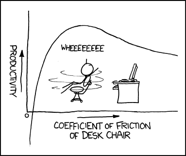 by Randall Munroe.
It will look nothing like this. This would be a poor fit for
your function.
:::
As a check, click on **landau** (which vaguely resembles the plot in
{numref}`Figure %s `) on the FitPanel's **Fit Function** pop-up menu and click on
**Fit** again; then try **expo** and fit again.
:::{note}
You may have to click on the **Fit** button more than once for the
button to "pick up" the click.
It looks like of these three choices (gaussian, landau, exponential),
the gaussian is the best functional form for this histogram. Take a look
at the "Chi2 / ndf" value in the statistics box on the histogram
("Chi2 / ndf" is pronounced "kye-squared per [number of] degrees of
freedom"). Do the fits again and observe how this number changes.
Typically, you know you have a good fit if this ratio is about 1.[^f32]
The FitPanel is good for gaussian distributions and other simple fits.
But for fitting large numbers of histograms (as you'd do in the
{ref}`advanced exercises` and the {ref}`expert exercises`) or for more
complex functions, you'll want to learn the following ROOT commands.
:::
To fit `hist1` to a gaussian, type the following command:[^f33]
[] hist1->Fit("gaus")
This does the same thing as using the FitPanel. You can close the
FitPanel; we won't be using it anymore.
Go back to the browser window and double-click on `hist2`.
:::{note}
You've probably already guessed by reading the x-axis label that I
created this histogram from the sum of two gaussian distributions. We're
going to fit this histogram by defining a custom function of our own.
:::
Define a user function with the following command:
[] TF1 func("mydoublegaus","gaus(0)+gaus(3)")
:::{note}
Note that the internal ROOT name of the function is "mydoublegaus",
but the name of the TF1 object is `func`.
What does `gaus(0)+gaus(3)` mean? You already know that the "gaus"
function uses three parameters. `gaus(0)` means to use the gaussian
distribution starting with parameter 0; `gaus(3)` means to use the
gaussian distribution starting with parameter 3. This means our user
function has six parameters: $P_0$, $P_1$, and $P_2$ are the
"constant", "mean", and "sigma" of the first gaussian, and $P_3$,
$P_4$, and $P_5$ are the "constant", "mean", and "sigma" of the
second gaussian.
:::
Let's set the values of $P_0$, $P_1$, $P_2$, $P_3$, $P_4$, and
$P_5$, and fit the histogram.[^f34]
[] func.SetParameters(5.,5.,1.,1.,10.,1.)
[] hist2->Fit("mydoublegaus")
It's not a very good fit, is it? This is because I deliberately picked a
poor set of starting values. Let's try a better set:
[] func.SetParameters(5.,2.,1.,1.,10.,1.)
[] hist2->Fit("mydoublegaus")
:::{note}
These simple fit examples may leave you with the impression that all
histograms in physics are fit with gaussian distributions. Nothing could
be further from the truth. I'm using gaussians in this class because
they have properties (mean and width) that you can determine by eye.
Chapter 5 of the [ROOT Users
Guide](https://root.cern/root/htmldoc/guides/users-guide/ROOTUsersGuide.html)
has a lot more information on fitting histograms, and a more realistic
example.
If you want to see how I created the file histogram.root, go to the UNIX
window and type:
> less ~seligman/root-class/CreateHist.C
In general, for fitting histograms in a real analysis, you'll have to
define your own functions and fit to them directly, with commands like:
[] TF1 func("myFunction","<...some parameterized TFormula...>")
[] func.SetParameters(...some values...)
[] myHistogram->Fit("myFunction")
For a simple gaussian fit to a single histogram, you can always go back
to using the FitPanel.
:::
:::{figure-md} curve_fitting-fig
:align: center
by Randall Munroe.
It will look nothing like this. This would be a poor fit for
your function.
:::
As a check, click on **landau** (which vaguely resembles the plot in
{numref}`Figure %s `) on the FitPanel's **Fit Function** pop-up menu and click on
**Fit** again; then try **expo** and fit again.
:::{note}
You may have to click on the **Fit** button more than once for the
button to "pick up" the click.
It looks like of these three choices (gaussian, landau, exponential),
the gaussian is the best functional form for this histogram. Take a look
at the "Chi2 / ndf" value in the statistics box on the histogram
("Chi2 / ndf" is pronounced "kye-squared per [number of] degrees of
freedom"). Do the fits again and observe how this number changes.
Typically, you know you have a good fit if this ratio is about 1.[^f32]
The FitPanel is good for gaussian distributions and other simple fits.
But for fitting large numbers of histograms (as you'd do in the
{ref}`advanced exercises` and the {ref}`expert exercises`) or for more
complex functions, you'll want to learn the following ROOT commands.
:::
To fit `hist1` to a gaussian, type the following command:[^f33]
[] hist1->Fit("gaus")
This does the same thing as using the FitPanel. You can close the
FitPanel; we won't be using it anymore.
Go back to the browser window and double-click on `hist2`.
:::{note}
You've probably already guessed by reading the x-axis label that I
created this histogram from the sum of two gaussian distributions. We're
going to fit this histogram by defining a custom function of our own.
:::
Define a user function with the following command:
[] TF1 func("mydoublegaus","gaus(0)+gaus(3)")
:::{note}
Note that the internal ROOT name of the function is "mydoublegaus",
but the name of the TF1 object is `func`.
What does `gaus(0)+gaus(3)` mean? You already know that the "gaus"
function uses three parameters. `gaus(0)` means to use the gaussian
distribution starting with parameter 0; `gaus(3)` means to use the
gaussian distribution starting with parameter 3. This means our user
function has six parameters: $P_0$, $P_1$, and $P_2$ are the
"constant", "mean", and "sigma" of the first gaussian, and $P_3$,
$P_4$, and $P_5$ are the "constant", "mean", and "sigma" of the
second gaussian.
:::
Let's set the values of $P_0$, $P_1$, $P_2$, $P_3$, $P_4$, and
$P_5$, and fit the histogram.[^f34]
[] func.SetParameters(5.,5.,1.,1.,10.,1.)
[] hist2->Fit("mydoublegaus")
It's not a very good fit, is it? This is because I deliberately picked a
poor set of starting values. Let's try a better set:
[] func.SetParameters(5.,2.,1.,1.,10.,1.)
[] hist2->Fit("mydoublegaus")
:::{note}
These simple fit examples may leave you with the impression that all
histograms in physics are fit with gaussian distributions. Nothing could
be further from the truth. I'm using gaussians in this class because
they have properties (mean and width) that you can determine by eye.
Chapter 5 of the [ROOT Users
Guide](https://root.cern/root/htmldoc/guides/users-guide/ROOTUsersGuide.html)
has a lot more information on fitting histograms, and a more realistic
example.
If you want to see how I created the file histogram.root, go to the UNIX
window and type:
> less ~seligman/root-class/CreateHist.C
In general, for fitting histograms in a real analysis, you'll have to
define your own functions and fit to them directly, with commands like:
[] TF1 func("myFunction","<...some parameterized TFormula...>")
[] func.SetParameters(...some values...)
[] myHistogram->Fit("myFunction")
For a simple gaussian fit to a single histogram, you can always go back
to using the FitPanel.
:::
:::{figure-md} curve_fitting-fig
:align: center
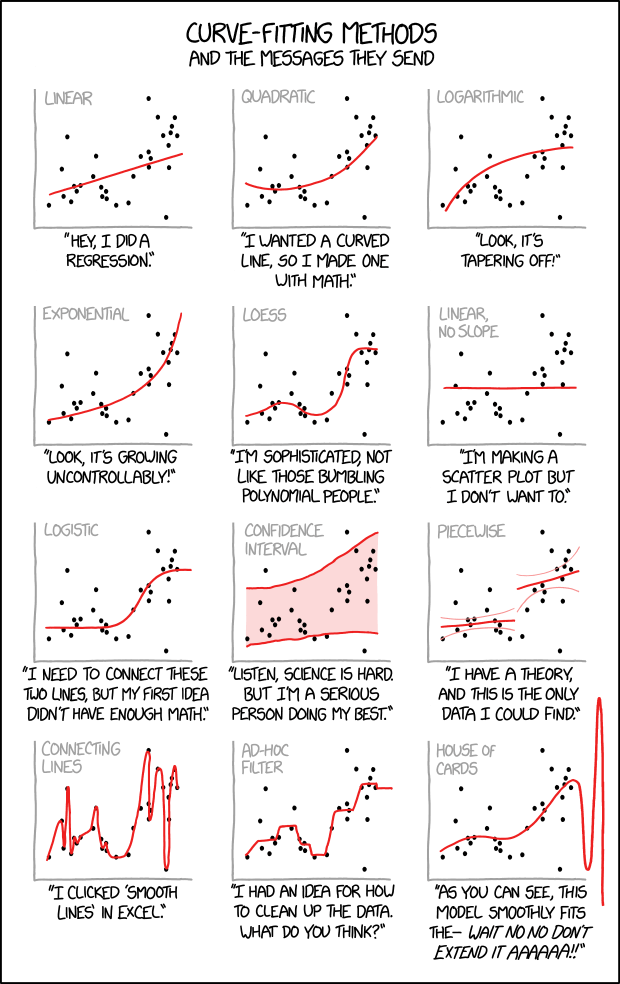 by Randall Munroe. Here are some possibilities for fitting plots using ROOT. If you choose to read the discussion on {ref}`statistics ` this cartoon may be funnier (or more tragic; such is the nature of physics).
:::
[^f31]: If you're going through this class and you can't login to a
system on the Nevis particle-physics Linux cluster, you'll have to
get the files from [my web site](https://www.nevis.columbia.edu/~seligman/root-class/files/).
If you want to get all the files from that directory at once, one
way is to use this UNIX command:
wget -r -np -nH --cut-dirs=2 -R "index.html*" \
https://www.nevis.columbia.edu/~seligman/root-class/files/
You may have to install the `wget` command on your system, since
it's often not installed by default.
Be aware that in that directory there are a lot of work files I
created to test things. There's more in there than just the files I
reference in my tutorials.
[^f32]: If you're not familiar with terms like "chi2" or "chi-squared"
there's a brief introduction to
{ref}`statistics ` in this tutorial.
[^f33]: What's the deal with the arrow "->" instead of the period? It's
because when you read in a histogram from a file, you get a pointer
instead of an object. This only matters in C++, not in Python. See
the section on {ref}`pointers ` for more information.
[^f34]: It may help to
cut-and-paste the commands from here into your ROOT window.
*Warning:* For now, don't fall into the trap of cutting-and-pasting
every command from this tutorial into ROOT. Save it for the more
complicated commands like `SetParameters` or file names like
`~seligman/root-class/AnalyzeVariables.C`. You want to get the
"feel" for issuing commands interactively (perhaps with the tricks
{ref}`you've learned `), and that won't happen if you
just type Ctrl-C/click/Ctrl-V over and over again.
When we get to {ref}`the notebook server`, you'll start cutting-and-pasting commands
into notebooks on a regular basis.
by Randall Munroe. Here are some possibilities for fitting plots using ROOT. If you choose to read the discussion on {ref}`statistics ` this cartoon may be funnier (or more tragic; such is the nature of physics).
:::
[^f31]: If you're going through this class and you can't login to a
system on the Nevis particle-physics Linux cluster, you'll have to
get the files from [my web site](https://www.nevis.columbia.edu/~seligman/root-class/files/).
If you want to get all the files from that directory at once, one
way is to use this UNIX command:
wget -r -np -nH --cut-dirs=2 -R "index.html*" \
https://www.nevis.columbia.edu/~seligman/root-class/files/
You may have to install the `wget` command on your system, since
it's often not installed by default.
Be aware that in that directory there are a lot of work files I
created to test things. There's more in there than just the files I
reference in my tutorials.
[^f32]: If you're not familiar with terms like "chi2" or "chi-squared"
there's a brief introduction to
{ref}`statistics ` in this tutorial.
[^f33]: What's the deal with the arrow "->" instead of the period? It's
because when you read in a histogram from a file, you get a pointer
instead of an object. This only matters in C++, not in Python. See
the section on {ref}`pointers ` for more information.
[^f34]: It may help to
cut-and-paste the commands from here into your ROOT window.
*Warning:* For now, don't fall into the trap of cutting-and-pasting
every command from this tutorial into ROOT. Save it for the more
complicated commands like `SetParameters` or file names like
`~seligman/root-class/AnalyzeVariables.C`. You want to get the
"feel" for issuing commands interactively (perhaps with the tricks
{ref}`you've learned `), and that won't happen if you
just type Ctrl-C/click/Ctrl-V over and over again.
When we get to {ref}`the notebook server`, you'll start cutting-and-pasting commands
into notebooks on a regular basis.