(first-notebook)=
# Your first notebook (10 minutes)
From the **New** menu, select Python 3. You'll see your first empty
cell, labeled `In [1]`. At the top of the page, you'll see that the
name of the notebook is **Untitled**. The first thing you should do when
creating a new notebook is to give it a new name. Go to the
**File** menu within the Jupyter page and select **Rename...**. Pick any
name you wish, such as `pythontest`.[^untitled]
[^untitled]: You don’t *have* to do this. But if you don’t, your home directory will soon be littered with notebooks named Untitled.ipynb, Untitled1.ipynb, Untitled2.ipynb, etc., and you won’t know what’s in any of them.
:::{figure-md} documents-fig
:class: align-center
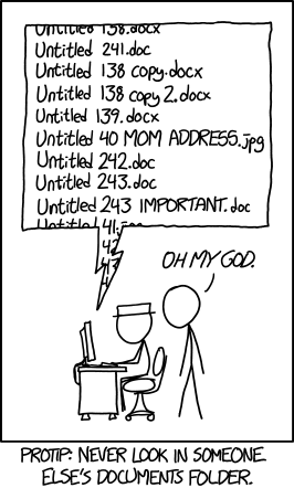 by Randall Munroe
:::
After you've renamed the notebook, go back to the Jupyter Home window.
You'll see the notebook file with the extension `.ipynb`.
Go back to the notebook window. Under the **Help** menu, take the **User
Interface Tour** (it's about a minute long). Note the **Keyboard
Shortcuts**.[^f50]
Cut-and-paste the following into that first cell.[^f51]
:::{code-block} python
from ROOT import TH1D, TCanvas
my_canvas = TCanvas("mycanvas","canvas title",800,600)
example = TH1D("example","example histogram",100,-3,3)
example.FillRandom("gaus",10000)
exomple.Draw("E")
my_canvas.Draw()
:::
:::{note}
This code is in Python, but after going through {ref}`the basics`
you can probably figure out what most of these lines are
supposed to do.
:::
To "execute" the contents of a given cell, hit SHIFT-ENTER with your
cursor in that cell. Do that now.
Oops! There's an error. Fix the error in the cell and hit SHIFT-ENTER
again.
:::{note}
Assuming there have been no mistakes, you should see a histogram
embedded in the web page.
There are also a couple of warning messages:
Warning in : Deleting canvas with same name: mycanvas
Warning in : Replacing existing TH1: example (Potential memory leak).
Let's think about what those messages mean. When you execute lines in a
cell, your environment doesn't "start fresh"; everything you defined
before is still there. ROOT is warning you that the `TCanvas` and the
histogram are being overridden.
In Python, you can usually ignore these warnings.
:::
Click in the next cell and cut-and-paste this line, then hit
SHIFT-ENTER:
exampleFit = example.Fit("gaus")
:::{note}
This next cell recognizes the histogram object you defined in
the previous cell. This gives you some idea of one feature of notebooks:
You can fiddle with something in a given cell until it does what you
want, then move on to the next phase of your task that depends on the
previous cell.
Wait a moment... We just added a fit to the histogram, but the plot
didn't change. Maybe we have to plot it again.
:::
Enter this line after the one you just pasted, or into a subsequent
cell, and hit SHIFT-ENTER:
example.Draw()
:::{note}
No new plot, and the plot above it still didn't change. What's wrong?
Nothing. Jupyter runs in a web browser, and browsers behave differently
than X-Windows (the underlying graphics protocol of UNIX). You may have
noticed that, unlike the ROOT plots in {ref}`the basics`, the shape of the cursor
doesn't change as you move it over the plot, and right-clicking on it
brings up a browser menu, not a ROOT one. If you right-click on the plot
and select **View Image**, you'll see that the plot is not a dynamic
object, but a static `.png` file.[^f52]
How do we get a plot? You probably guessed the answer from what I had in
the first cell. Paste the following line after that last `Draw()`
command, or in a new cell:
my_canvas.Draw()
Finally, you see the histogram with the fit superimposed.
{ref}`Remember `: ROOT
plots everything in a canvas. In Jupyter, a `TCanvas` is not automatically
drawn when its underlying plot updates. You have to explicitly draw the
`TCanvas` yourself. That's why the first example contains the lines:
my_canvas = TCanvas("mycanvas","canvas title",800,600)
# ... stuff ...
my_canvas.Draw()
I had to define the `TCanvas` that would be used as the "target" of any
Draw commands, then Draw that `TCanvas` in order for the plot to be
displayed.[^f53]
:::
[^f50]: Here are more [Jupyter hints](https://www.dataquest.io/blog/jupyter-notebook-tips-tricks-shortcuts/).
Some of those tips won't work on the Nevis systems; e.g., you can't
install new packages on the Nevis notebook server. The last tip, on
different ways to share notebooks, will be helpful to those who work
with folks who don't use Jupyter.
[^f51]: You can type it in manually if you want, but (a) that's a lot of
typing, and (b) you have to make sure you get each character correct
for the sake of this example.
[^f52]: "PNG" stands for Portable Network Graphics. It's a standardized
format for uncompressed images to be sent over the web. Jupyter uses
that format instead of GIF because the GIF algorithm is patented.
[^f53]: Since we haven't had to explicitly define our canvases before, I
should mention: the canvas name and title are usually not important;
the name only matters if you were to write the canvas to a file, and
the canvas title is rarely displayed (as opposed to the histogram
title, which appears at the top of the plot).
What matters is the size of the canvas. Here, I used 800 pixels wide
and 600 pixels tall, which is the size of our old friend `c1`
that's automatically defined if you don't define a canvas yourself.
I could have defined the canvas using only defaults with
my_canvas = TCanvas()
but I thought that might be even more confusing to see for the first
time.
by Randall Munroe
:::
After you've renamed the notebook, go back to the Jupyter Home window.
You'll see the notebook file with the extension `.ipynb`.
Go back to the notebook window. Under the **Help** menu, take the **User
Interface Tour** (it's about a minute long). Note the **Keyboard
Shortcuts**.[^f50]
Cut-and-paste the following into that first cell.[^f51]
:::{code-block} python
from ROOT import TH1D, TCanvas
my_canvas = TCanvas("mycanvas","canvas title",800,600)
example = TH1D("example","example histogram",100,-3,3)
example.FillRandom("gaus",10000)
exomple.Draw("E")
my_canvas.Draw()
:::
:::{note}
This code is in Python, but after going through {ref}`the basics`
you can probably figure out what most of these lines are
supposed to do.
:::
To "execute" the contents of a given cell, hit SHIFT-ENTER with your
cursor in that cell. Do that now.
Oops! There's an error. Fix the error in the cell and hit SHIFT-ENTER
again.
:::{note}
Assuming there have been no mistakes, you should see a histogram
embedded in the web page.
There are also a couple of warning messages:
Warning in : Deleting canvas with same name: mycanvas
Warning in : Replacing existing TH1: example (Potential memory leak).
Let's think about what those messages mean. When you execute lines in a
cell, your environment doesn't "start fresh"; everything you defined
before is still there. ROOT is warning you that the `TCanvas` and the
histogram are being overridden.
In Python, you can usually ignore these warnings.
:::
Click in the next cell and cut-and-paste this line, then hit
SHIFT-ENTER:
exampleFit = example.Fit("gaus")
:::{note}
This next cell recognizes the histogram object you defined in
the previous cell. This gives you some idea of one feature of notebooks:
You can fiddle with something in a given cell until it does what you
want, then move on to the next phase of your task that depends on the
previous cell.
Wait a moment... We just added a fit to the histogram, but the plot
didn't change. Maybe we have to plot it again.
:::
Enter this line after the one you just pasted, or into a subsequent
cell, and hit SHIFT-ENTER:
example.Draw()
:::{note}
No new plot, and the plot above it still didn't change. What's wrong?
Nothing. Jupyter runs in a web browser, and browsers behave differently
than X-Windows (the underlying graphics protocol of UNIX). You may have
noticed that, unlike the ROOT plots in {ref}`the basics`, the shape of the cursor
doesn't change as you move it over the plot, and right-clicking on it
brings up a browser menu, not a ROOT one. If you right-click on the plot
and select **View Image**, you'll see that the plot is not a dynamic
object, but a static `.png` file.[^f52]
How do we get a plot? You probably guessed the answer from what I had in
the first cell. Paste the following line after that last `Draw()`
command, or in a new cell:
my_canvas.Draw()
Finally, you see the histogram with the fit superimposed.
{ref}`Remember `: ROOT
plots everything in a canvas. In Jupyter, a `TCanvas` is not automatically
drawn when its underlying plot updates. You have to explicitly draw the
`TCanvas` yourself. That's why the first example contains the lines:
my_canvas = TCanvas("mycanvas","canvas title",800,600)
# ... stuff ...
my_canvas.Draw()
I had to define the `TCanvas` that would be used as the "target" of any
Draw commands, then Draw that `TCanvas` in order for the plot to be
displayed.[^f53]
:::
[^f50]: Here are more [Jupyter hints](https://www.dataquest.io/blog/jupyter-notebook-tips-tricks-shortcuts/).
Some of those tips won't work on the Nevis systems; e.g., you can't
install new packages on the Nevis notebook server. The last tip, on
different ways to share notebooks, will be helpful to those who work
with folks who don't use Jupyter.
[^f51]: You can type it in manually if you want, but (a) that's a lot of
typing, and (b) you have to make sure you get each character correct
for the sake of this example.
[^f52]: "PNG" stands for Portable Network Graphics. It's a standardized
format for uncompressed images to be sent over the web. Jupyter uses
that format instead of GIF because the GIF algorithm is patented.
[^f53]: Since we haven't had to explicitly define our canvases before, I
should mention: the canvas name and title are usually not important;
the name only matters if you were to write the canvas to a file, and
the canvas title is rarely displayed (as opposed to the histogram
title, which appears at the top of the plot).
What matters is the size of the canvas. Here, I used 800 pixels wide
and 600 pixels tall, which is the size of our old friend `c1`
that's automatically defined if you don't define a canvas yourself.
I could have defined the canvas using only defaults with
my_canvas = TCanvas()
but I thought that might be even more confusing to see for the first
time.