Walkthrough: Fitting to a user-defined function

(10 minutes)

Go back to the browser window and double-click on hist2.

Note

You’ve probably already guessed by reading the x-axis label that I created this histogram from the sum of two Gaussian distributions. We’re going to fit this histogram by defining a custom function of our own.

Define a user function with the following command:

[] TF1 func("mydoublegaus","gaus(0)+gaus(3)")

Note

Note that the internal ROOT name of the function is “mydoublegaus”, but the name of the TF1 object is func.

What does gaus(0)+gaus(3) mean? You already know that the “gaus” function uses three parameters. gaus(0) means to use the Gaussian distribution starting with parameter 0; gaus(3) means to use the Gaussian distribution starting with parameter 3. This means our user function has six parameters: \(P_0\), \(P_1\), and \(P_2\) are the “constant”, “mean”, and “sigma” of the first Gaussian, and \(P_3\), \(P_4\), and \(P_5\) are the “constant”, “mean”, and “sigma” of the second Gaussian.

Let’s set the values of \(P_0\), \(P_1\), \(P_2\), \(P_3\), \(P_4\), and \(P_5\), and fit the histogram.1

[] func.SetParameters(5.,5.,1.,1.,10.,1.)
[] hist2->Fit("mydoublegaus")

It’s not a very good fit, is it? This is because I deliberately picked a poor set of starting values. Let’s try a better set:

[] func.SetParameters(5.,2.,1.,1.,10.,1.)
[] hist2->Fit("mydoublegaus")

Note

These simple fit examples may leave you with the impression that all histograms in physics are fit with Gaussian distributions. Nothing could be further from the truth. I’m using Gaussians in this class because they have properties (mean and width) that you can determine by eye.

Chapter 5 of the ROOT Users Guide has a lot more information on fitting histograms, and a more realistic example.

If you want to see how I created the file histogram.root, go to the UNIX window and type:

> less ~seligman/root-class/CreateHist.C

In general, for fitting histograms in a real analysis, you’ll have to define your own functions and fit to them directly, with commands like:

[] TF1 func("myFunction","<...some parameterized TFormula...>")
[] func.SetParameters(...some values...)
[] myHistogram->Fit("myFunction")

For a simple Gaussian fit to a single histogram, you can always go back to using the FitPanel.

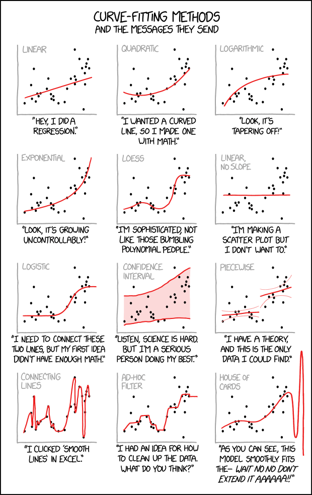
Figure 14: http://xkcd.com/2048 by Randall Munroe. Here are some possibilities for fitting plots using ROOT. If you choose to read the discussion on statistics this cartoon may be funnier (or more tragic; such is the nature of physics).

---

1

It may help to cut-and-paste the commands from here into your ROOT window.

Warning: For now, don’t fall into the trap of cutting-and-pasting every command from this tutorial into ROOT. Save it for the more complicated commands like SetParameters or file names like ~seligman/root-class/AnalyzeVariables.C. You want to get the “feel” for issuing commands interactively (perhaps with the tricks you’ve learned), and that won’t happen if you just type Ctrl-C/click/Ctrl-V over and over again.

When we get to The Notebook Server, you’ll start cutting-and-pasting commands into notebooks on a regular basis.