Chi-squared
It’s rare in physics to perform an analysis task and see nice smooth curves like those in Figure 89. For the most part, you make histograms of values, as in my introductory talk. Such a plot might look something like this:1
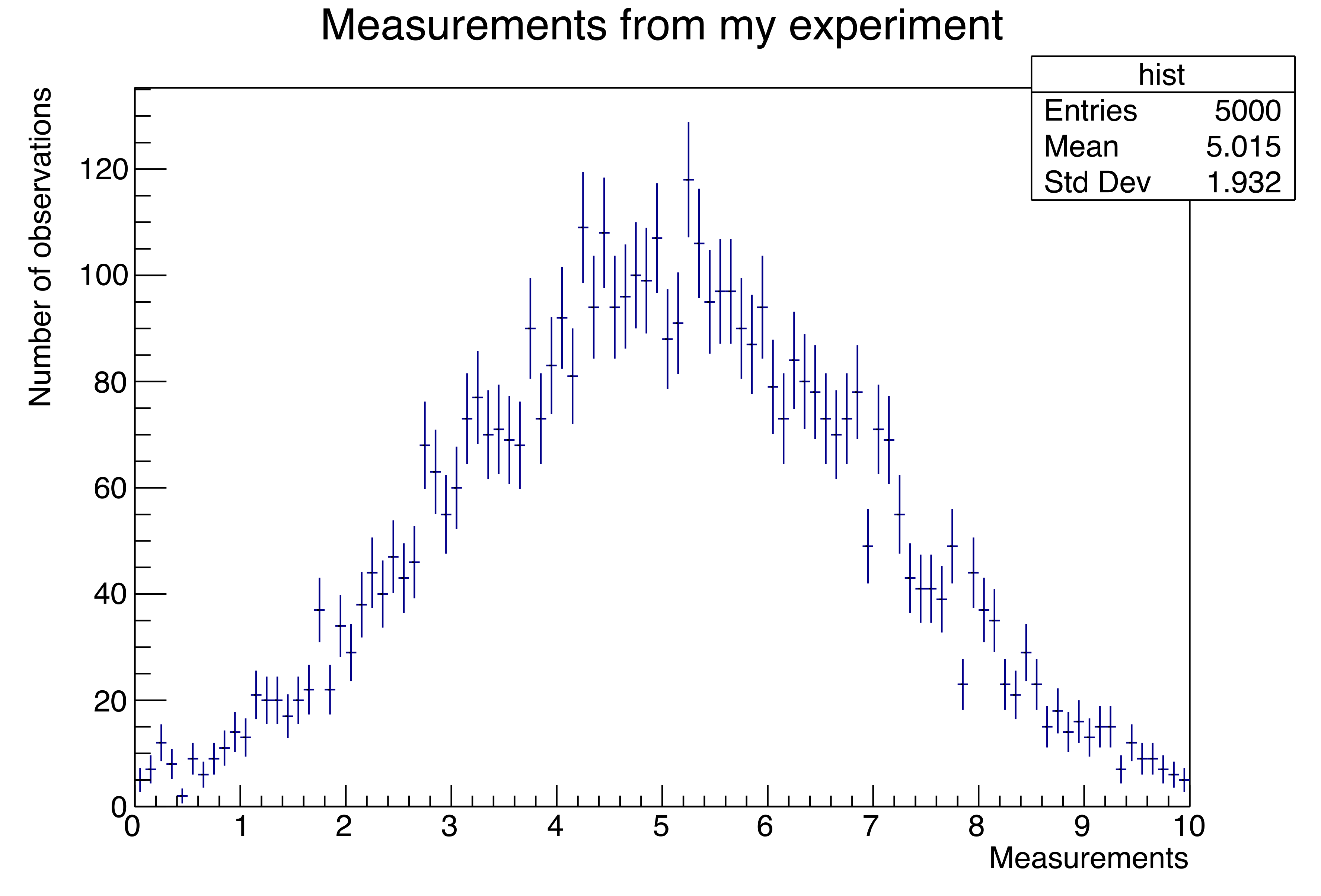
Figure 93: A typical histogram that you might create during a data analysis.
Suppose you want to test whether the above distribution of data was generated according to a Gaussian distribution. The usual test in physics is to perform a “fit”: fiddle with the Gaussian’s parameters \(A\), \(\mu\), and \(\sigma\) (typically called “amplitude”, “mean”, and “sigma” respectively) until the function best fits those data points.
The mathematical method for performing such a fit starts with computing
a quantity denoted as
where:
\(i\) means the \(i\)-th bin of the histogram (more generally, the \(i\)-th data point you’ve gathered).
\(y_{i}\) means the data in (or the value of) the \(i\)-th bin of the histogram.
\(e_{i}\) means the error in the \(i\)-th bin of the histogram (i.e., the size of the error bars).
\(f\left( x_{i};p_{j} \right)\) means to compute the value of the function at \(x_{i}\) (the value on the \(x\)-axis of the center of bin \(i\)) given some assumed values of the parameters \(p_{0},p_{1},p_{2}\ldots p_{j}\).
The process of “fitting” means to test different values of the parameters until you find those that minimize the value of \(\chi^{2}\).
This probably sounds quite involved. Indeed, it can be. Fortunately, physicists and mathematicians have developed many tools to relieve the computational tedium of much of this process. As you will learn in The Basics (if you jumped here) or learned in The Basics (if you’re reading this tutorial from beginning to end), fitting the histogram in Figure 93 to a Gaussian distribution is a matter of a couple of mouse clicks:
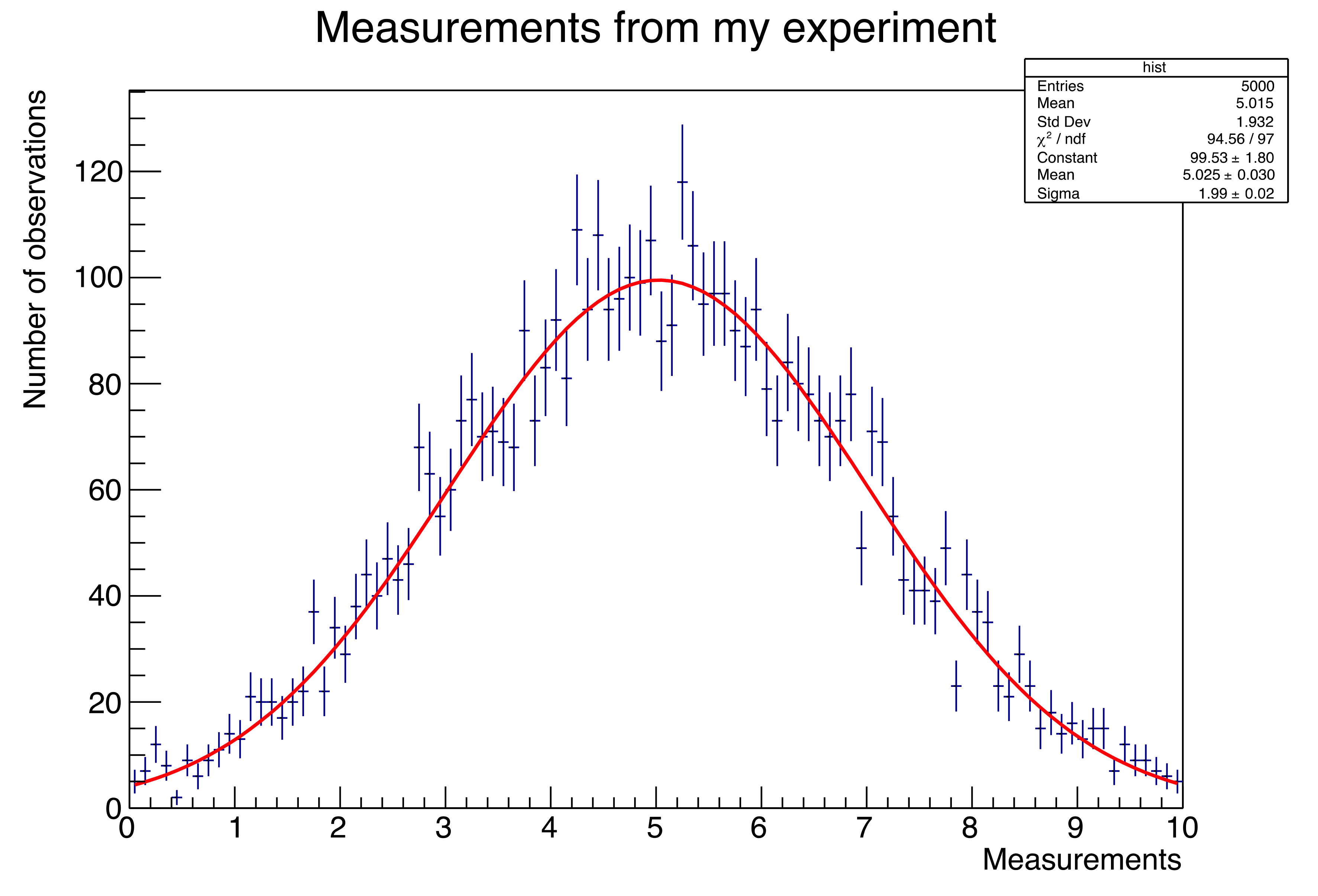
Figure 94: It looks like a Gaussian function is a reasonable assumption for the underlying distribution of our data. In this case, I knew this to be true because of how I generated the “data” in the histogram. You (will do)/(have done)/(will have done) the same thing in The Basics.
Since you’re a scientist, you may ask “How does ROOT fit functions?”
The answer has to do with a general mathematical technique called
“function minimization”; in this case, minimizing the value of
I should mention that you don’t always fit a function to your data using a \(\chi^{2}\)calculation. That’s good enough if the distribution of your data within each individual bin is Gaussian; it’s reasonably true for the fits associated with this tutorial.
However, in physics you can have data vs. function comparisons for which the underlying data within a bin is not Gaussian. This frequently occurs with fits that include Systematic errors.
For another example, look at Figure 94, and consider the bins on the far left- and right-hand sides of the plot. The error bars are simply the square root of the number of events in the bin, which is a reasonable approximation for a Gaussian. But the number of events in those left/right bins is less than ten, which you know from Figure 91 should be represented by a Poisson distribution.4
For these cases you may need to use a “log-likelihood” test. I won’t discuss this further5\(^,\)6 but it’s important that you know it exists.
For more on this topic, I prepared a Jupyter notebook on how to use a general-purpose function minimization program called Minuit from within Python and apply it to histograms I created using ROOT.7 If you’re interested in this (or writing minimization routines), you can view a static version of my Minuit notebook, or you can copy the file:
cp ~seligman/root-class/minuit-class.ipynb $PWD
- 1
If you jumped here from The Basics, you’re going to make your own plots similar to the next couple of figures.
- 2
That’s “chi” with the ch pronounced like a k; the word rhymes with sky. If you pronounce it “chee” with a soft ch, folks at Nevis will think you’re talking about a scientist named Qi.
- 3
If you’ve studied machine learning, some of this will sound familiar; e.g., here the “cost function” is
\(\chi^{2}\). The procedure is still to follow deepest descent of the gradient of a function to locate a minimum. However, the nitty-gritty details aren’t the same because a \(\chi^{2}\) fit is a different problem; I wouldn’t use Tensorflow to fit a Gaussian to experimental data!- 4
Remember that footnote back in Working with Histograms? Neither do I. Wait… I think it was the one that talked about varying bin widths in a histogram. Now you know why that can be a good idea: so that all of the bins have enough events that they can reasonably approximated by a Gaussian distribution, and a \(\chi^{2}\) fit would be appropriate.
- 5
…because I don’t fully understand it myself. Maybe, at the end of your research work at Nevis, you’ll teach me!
- 6
There’s a package in ROOT called RooFit that easily performs log-likelihood fits. Another important feature is that RooFit can perform fits on a set of individual data points, instead of requiring that the data be binned in a histogram.
- 7
If you don’t know what a “Jupyter notebook” is, it means you haven’t yet reached The Notebook Server in this tutorial.