Chi-squared per degree of freedom
Let’s suppose your supervisor asks you to perform a fit on some data. They may ask you about the chi-squared of that fit. However, that’s short-hand; what they really want to know is the chi-squared per the number of degrees of freedom.
Take a careful look at the text box in the upper right-hand corner of Figure 94. One of the lines in that box is “\(\chi^{2}\) / ndf”. You’ve already figured that it’s short for “chi-squared per the number of degrees of freedom” but what does that actually mean?
Take another look at Equation (6) for the Gaussian function:

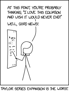
Figure 95: https://xkcd.com/2605/ by Randall Munroe. The \(\chi^{2}\) calculation is not a Taylor series! But given enough data points…
As I mentioned before, within each histogram bin \(i\) the data is assumed to form a little Gaussian distribution of its own with a mean of \(y_i\). The \(e_i\) acts as a scale of the difference between \(y_i\) and the function \(f(x)\). So if \(f(x)\) is a reasonable approximation to \(y_{i}\), \(\frac{\left( y_{i} - f(x) \right)}{e_{i}}\) will be around ±1. You add up those “1”s for each of the bins, and you might anticipate that \(\chi^{2}\) will be roughly equal to \(i\), the number of bins.
That doesn’t tell the whole story. There are three “free parameters” in the fit: \(A,\mu,\sigma\). They’re going to be varied to make the chi-squared smaller. The net effect is that total number of “degrees of freedom” for minimizing the \(\chi^{2}\) is:
DOF = number of data points – number of free parameters in the function
The histogram in Figure 94 has 100 bins, and a Gaussian function has three parameters. If you look at the figure again, you’ll see \(\chi^{2}\) / ndf = 94.56 / 97. It looks like ROOT knows how to count the degrees of freedom, at least for simple functions and histogram fits. If you’re using a more sophisticated fitting program like Minuit, you may have to figure out the DOF yourself.
So far so good, but would it better if the \(\chi^{2}\) were even lower? No, it wouldn’t!
Statisticians have studied the question: What is the probability that a randomly-generated set of data came from a particular underlying distribution? If you look around the web, you’ll find tables that compute this probability for a given \(\chi^{2}\) and ndf. When you get to more than a couple dozen ndf, there’s a simpler test: see if the ratio \(\chi^{2}\) / ndf is around 1. For the particular fit in Figure 94, the value of \(\chi^{2}\) / ndf = 94.56 / 97 is reasonably close to 1; your supervisor would probably accept it.
What might cause \(\chi^{2}\) / ndf to be much greater than 1?
There’s something wrong in the routine that’s calculating \(\chi^{2}\), either in the code or the underlying model. That probably won’t happen if you’re fitting histograms in ROOT with simple functions, but I can’t tell you the number of days I’ve spent sweating over a chi-square calculation that I wrote.1
The model that’s being assumed for the function does not have enough freedom or has the wrong form to fit the data. This does not mean you can just throw additional parameters into the function for the sake of improving the \(\chi^{2}\)! 2
The error bars for your data are too small; in other words, there are additional sources of error (possibly systematic error) which you have not yet included.
Function-minimization programs can get “stuck” in a local minimum that’s not the actual true minimum; there’s an example of that in The Basics (and in that Minuit notebook I described above).
What might cause \(\chi^{2}\) / ndf to be much less than 1?
Again, something wrong in the \(\chi^{2}\) calculation.
Too many free parameters in the function you’re using to fit. For an extreme example, consider what would happen if we tried to fit Figure 94 with a 100-degree polynomial. Of course, that function would be able to go through the middle of every \(y_i\) in the plot and the resulting \(\chi^{2}\) would be close to zero.3
The error bars for your data are too large. This can happen if you’re not careful in how you add up your errors; if you simply add all your errors in quadrature \(\left( \sqrt{ {\sigma_{0}^{2} + \sigma_{1}^{2} + \sigma_{2}^{2} + \ldots} } \right)\) you may have overlooked that some of your errors are correlated; i.e., there are terms \(\sigma_{i}\sigma_{j}\) where \(i \neq j\). If that’s the case, you have to calculate \(\chi^{2}\) with an extension of Equation (6) using a covariance matrix.
Someone has gone wrong in your data-analysis process and you’re “tuning” the data to the model you want to fit.4

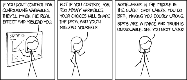
Figure 96: https://xkcd.com/2560/ by Randall Munroe
- 1
…or worse, someone else wrote, then graduated quickly before anyone could ask troublesome questions.
- 2
In case you think I’m joking: This actually happened during the analysis effort of my thesis experiment. No, I wasn’t the one who did it. The issue remained unnoticed for a few years before I uncovered the problem; fortunately, we hadn’t published any papers based on that erroneous fit.
- 3
See Figure 14 for an example.
- 4
This can happen accidentally, but there are times it’s deliberate. Five decades after the death of the monk Gregor Mendel, a statistical analysis of his results showed that he was faking his data to agree with his model of genetic inheritance. As it turned out, his model was correct. That makes him the luckiest fraud in the history of science.